NEMO: Atlantic Margin Model

This tutorial gives an end-to-end example on how to install and then run NEMO-ERSEM on the 7 km Atlantic Margin Model 7 (AMM7) domain using a high performance computing (HPC) machine. Here we have used UK National Supercomputing Service ARCHER2 with a singularity container with NEMO-ERSEM installed on it.

This tutorial is based on utilising a singularity container with a NEMO-ERSEM install within. The configuration scripts used in the installation can be found here. You will also need access to the shared folder within the ARCHER2 project id n01 to obtain the forcing files.

Obtaining NEMO-ERSEM container

The key packages that are installed into NEMO-ERSEM container are:

NEMO, ERSEM and FABM are freely available on GitHub and XIOS is available through the NEMO consortium svn server. Full instructions how to build the container can be found here. We note these instructions are based on the “Containerisation of NEMO Employing Singularity” (CoNES) repository.

Running the container on ARCHER2

The instructions to generate the slurm HPC scheduling scripts can be found here. These are used to run the model on ARCHER2.

The scripts generated via mkslurm require two executables, namely xios_server.exe and nemo. In a native installation, one would simply link the XIOS and NEMO executables to xios_server.exe and nemo. However, when using the singularity container, you are required to create xios_server.exe and nemo executables based on the following bash script:

Example script to run container. User is required to change [RUNING-DIR] and [INPUT-DIR] to the corresponding directories, and [NEMO-XIOS] to either nemo or xios.

#! /bin/bash
BIND_OPTS="-B [RUNING-DIR],"
BIND_OPTS="${BIND_OPTS}[INPUT-DIR],"
BIND_OPTS="${BIND_OPTS}/usr/lib64/liblustreapi.so:/opt/lib64/liblustreapi.so,"
BIND_OPTS="${BIND_OPTS}/usr/lib64/liblustreapi.so.1:/opt/lib64/liblustreapi.so.1,"
BIND_OPTS="${BIND_OPTS}/usr/lib64/liblustreapi.so.1.0.0:/opt/lib64/liblustreapi.so.1.0.0,"
BIND_OPTS="${BIND_OPTS}/opt/cray/libfabric/1.11.0.4.71/lib64/:/opt/fabric,"
BIND_OPTS="${BIND_OPTS}/usr/lib64/libpals.a:/opt/lib64/libpals.a,"
BIND_OPTS="${BIND_OPTS}/usr/lib64/libpals.so:/opt/lib64/libpals.so,"
BIND_OPTS="${BIND_OPTS}/usr/lib64/libpals.so.0:/opt/lib64/libpals.so.0,"
BIND_OPTS="${BIND_OPTS}/usr/lib64/libpals.so.0.0.0:/opt/lib64/libpals.so.0.0.0,"
BIND_OPTS="${BIND_OPTS}/opt/cray/pe/mpich/8.1.9/ofi/gnu/9.1:/opt/mpi/install/,"
BIND_OPTS="${BIND_OPTS}/opt/cray/pe/pmi/6.0.13/lib,"
BIND_OPTS="${BIND_OPTS}/var/spool/slurmd/mpi_cray_shasta"

export SINGULARITYENV_LD_LIBRARY_PATH=/opt/hdf5/install/lib:$SINGULARITYENV_LD_LIBRARY_PATH
export SINGULARITYENV_LD_LIBRARY_PATH=/opt/mpi/install/lib-abi-mpich:$SINGULARITYENV_LD_LIBRARY_PATH
export SINGULARITYENV_LD_LIBRARY_PATH=/.singularity.d/libs:$SINGULARITYENV_LD_LIBRARY_PATH
export SINGULARITYENV_LD_LIBRARY_PATH=/opt/cray/pe/pmi/6.0.13/lib:$SINGULARITYENV_LD_LIBRARY_PATH
export SINGULARITYENV_LD_LIBRARY_PATH=/opt/lib64:$SINGULARITYENV_LD_LIBRARY_PATH
export SINGULARITYENV_LD_LIBRARY_PATH=/opt/fabric:$SINGULARITYENV_LD_LIBRARY_PATH
export LD_LIBRARY_PATH=/opt/hdf5/install/lib
export OMP_NUM_THREADS=1

singularity run ${BIND_OPTS} --home [RUNING-DIR] nemo.sif [NEMO-XIOS]

The CoNES documentation gives additional information on how to run NEMO singularity containers.

Example output from NEMO-ERSEM

To visualise NEMO output, we recommend using nctoolkit. A basic example of how to use nctoolkit is given below. Within the documentation of nctoolkit one will find additional example uses.

Example plotting script using nctoolkit, user is required to change [PATH_TO_NETCDF_FILE] and [VARIABLE] to the exact location of the NEMO output and the variable to be plotted, respectively.

import nctoolkit as nc

# path to netCDF file
ff = [PATH_TO_NETCDF_FILE]
ds = nc.open_data(ff)

# removes colours from land values
ds.set_missing(0)

# draws the outline of the land
ds.fix_nemo_ersem_grid()

# selects the final timestep for plotting
ds.select(time=[len(ds.times)-1])

# plots the variable. Note, the colour bar will change for each plot since autoscale
# is set to False
plot = ds.plot([VARIABLE], autoscale=False)

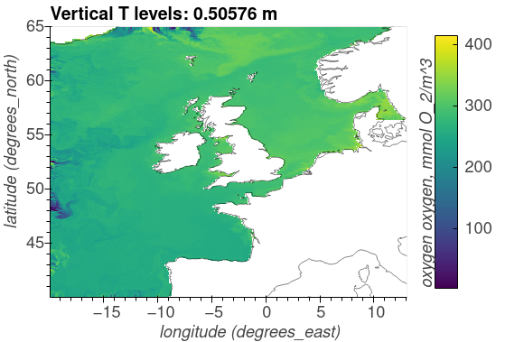
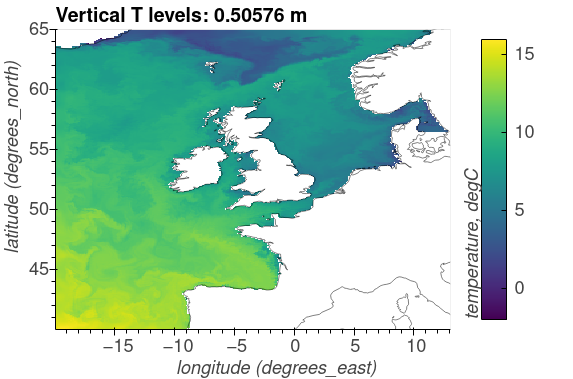
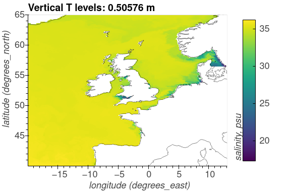
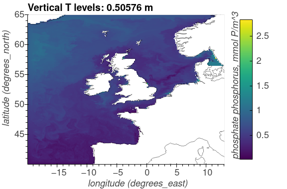
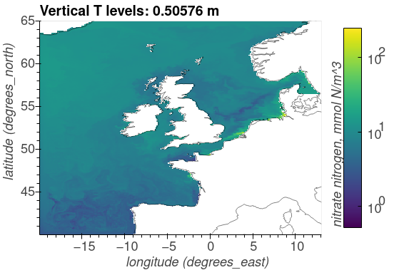
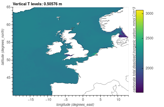
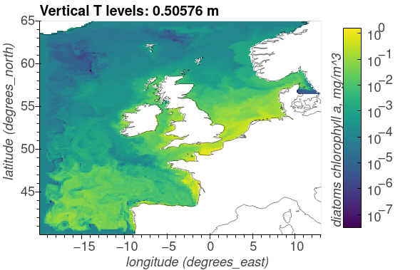
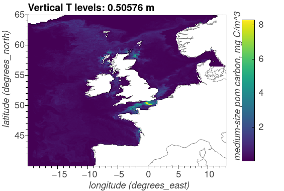
The following plots show the surface distributions of a subset of variables from the NEMO-ERSEM simulation on the AMM7 domain.

Note

The plots below are snapshots take from the model output at 30/01/2005.